November 6, 2024

Build Neural Network from Scratch in Python

Introduction

Neural networks are a class of machine learning models inspired by the structure of the human brain. They consist of layers of interconnected nodes (neurons) that can learn and generalize complex patterns in data. These networks are trained by adjusting the connections (weights) between neurons based on the data they process. Neural networks are widely used in fields like image recognition, natural language processing, and more.

The goal of this post is to demonstrate how to build a simple neural network from scratch that can recognize handwritten digits from the MNIST dataset, a common benchmark in machine learning. We’ll guide you through each component of the neural network and cover the theory and code needed to understand its learning process.

Dataset

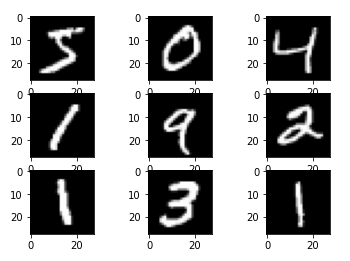
The MNIST dataset contains 60,000 training images and 10,000 test images of handwritten digits (0–9). Each image is 28x28 pixels, resulting in a 784-pixel input per image. The images are grayscale, so each pixel value ranges from 0 to 255, where 0 represents a white pixel and 255 represents a black one.

To prepare the data, each image is flattened into a 784-dimensional vector. This enables us to input it directly into our neural network, which has 784 input neurons. We also normalize the pixel values by dividing by 255, ensuring each input value falls between 0 and 1.

Neural Network Structure

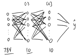
Our neural network has three layers:

1. Input Layer: Consists of 784 neurons, one for each pixel in the flattened 28x28 image.

2. Hidden Layer: Contains 10 neurons with ReLU (Rectified Linear Unit) activation to introduce non-linearity. This layer helps the network learn more complex patterns within the data.

3. Output Layer: Has 10 neurons, one for each digit (0–9). The softmax activation function is applied to this layer to interpret the network’s output as probabilities for each digit class.

The 784-10-10 architecture was chosen as a balance between simplicity and effectiveness. It’s simple enough to code from scratch and yet powerful enough to classify MNIST digits with reasonable accuracy.

How Neural Networks Learn

The learning process of a neural network involves passing data through the network to make predictions, calculating the error in these predictions, and then adjusting the network’s parameters to reduce this error. The main stages are forward propagation, activation functions, backward propagation, and gradient descent.

Forward Propagation

In forward propagation, data flows through the network from the input layer to the output layer. Each layer performs a set of computations to transform the input data and produce an output that is passed to the next layer. This process involves linear transformations and activation functions.

For example, in our network:

1. We start with the input $X$ (in this case, each image flattened into a 784-length vector).

2. This input is transformed by a set of weights and biases in each layer. For the first layer, the transformation is:

   $Z_1 = W_1 \cdot X + b_1$

   where  $W_1$  and  $b_1$  are the weights and biases for the first layer, respectively. This produces an intermediate result $Z1$ that is passed through an activation function to introduce non-linearity.

3. For the hidden layer, we use ReLU as the activation function. After ReLU, we get $A1$, which represents the activated output of the first layer:

   $A_1 = \text{ReLU}(Z_1)$

4. The next layer performs a similar transformation with a different set of weights and biases:

   $Z_2 = W_2 \cdot A_1 + b_2$

5. Finally, the output Z2 is passed through the softmax activation function to get probabilities for each of the 10 digits (0–9). This output is represented as $A2$:

   $A_2 = \text{softmax}(Z_2)$

The final result $A2$ is an array of probabilities representing the model’s confidence in each class (digit).

Activation Functions: ReLU and Softmax

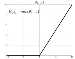
• ReLU (Rectified Linear Unit) is an activation function used to introduce non-linearity. It is defined as:

  $\text{ReLU}(Z) = \max(0, Z)$

  ReLU outputs the input $Z$ if it is positive, and zero otherwise. This non-linearity allows the network to capture complex patterns, as it effectively ignores negative values while preserving positive ones. ReLU helps prevent the “vanishing gradient” problem that can make training deep networks difficult.

  

• Softmax is an activation function applied to the output layer to interpret the model’s predictions as probabilities. It transforms the raw output values into probabilities that sum to 1, making it suitable for multi-class classification. The softmax function for an output vector $Z$ is defined as:

  $\text{softmax}(Z_i) = \frac{e^{Z_i}}{\sum_{j} e^{Z_j}}$

  where  $e^{Z_i}$  is the exponential function applied to each element of $Z$. Softmax emphasizes the largest values in $Z$, making it easier for the model to confidently pick one class.

Backward Propagation

Backward propagation calculates how much each weight and bias contributed to the error in the model’s predictions. Using these calculations, the network can “learn” by adjusting the weights and biases to reduce this error.

1. First, we calculate the error at the output layer by comparing A2 (the predicted output) with the true labels Y, encoded as one-hot vectors. The difference between A2 and Y gives us dZ2, the gradient of the loss with respect to Z2.

   $dZ_2 = A_2 - \text{one\_hot\_Y}$

2. We then calculate the gradients of the weights and biases for the output layer (dW2, db2). These gradients tell us how much to adjust the weights and biases to reduce the error.

   $dW_2 = \frac{1}{m} dZ_2 \cdot A_1^T$

   $db_2 = \frac{1}{m} \sum dZ_2$

3. Next, we propagate the error backward to the hidden layer. Using the derivative of the ReLU function, we calculate dZ1, the gradient of the loss with respect to Z1.

   $dZ_1 = W_2^T \cdot dZ_2 \cdot \text{ReLU\_deriv}(Z_1)$

4. We then calculate dW1 and db1 for the first layer:

   $dW_1 = \frac{1}{m} dZ_1 \cdot X^T$

   $db_1 = \frac{1}{m} \sum dZ_1$

Updating Parameters

After calculating the gradients, we use gradient descent to update the parameters, moving in the direction that reduces the network’s error. This is achieved by adjusting the weights and biases using the gradients calculated during backward propagation. The formulas for updating each parameter are as follows:

where  $\alpha$  is the learning rate, a hyperparameter that controls how large the adjustments are in each iteration. Lower values of  $\alpha$  lead to smaller, more precise updates, while higher values can speed up training but may risk overshooting the minimum error.

Each parameter update reflects the network’s learning from the data. By repeating these updates over many iterations, the network minimizes the error and improves its ability to make accurate predictions.

Full code

1. Import Libraries and Prepare the Dataset

   In this step, we import necessary libraries and prepare the MNIST data for training.

   1 2 3 4 5 6 7 8 9 10 from keras.datasets import mnist import numpy as np import matplotlib.pyplot as plt # Load and preprocess dataset (x_train, y_train), (x_test, y_test) = mnist.load_data() n = x_train[0].shape[0] * x_train[0].shape[0] # Flatten 28x28 images to 784-length vector m = x_train.shape[0] # Number of training examples x_train = x_train.reshape(x_train.shape[0], n).T / 255 # Normalize pixel values to 0-1 x_test = x_test.reshape(x_test.shape[0], n).T / 255

2. Initialize Parameters

   This function initializes the weights and biases for each layer of the network with small random values.

   1 2 3 4 5 6 def init_params(): W1 = np.random.rand(10, 784) - 0.5 # Weights for hidden layer b1 = np.random.rand(10, 1) - 0.5 # Biases for hidden layer W2 = np.random.rand(10, 10) - 0.5 # Weights for output layer b2 = np.random.rand(10, 1) - 0.5 # Biases for output layer return W1, b1, W2, b2

3. Define Activation Functions

   Here, we define the ReLU and softmax activation functions. ReLU introduces non-linearity in the hidden layer, and softmax outputs probabilities for each class in the output layer.

   1 2 3 4 5 6 def ReLU(Z): return np.maximum(Z, 0) def softmax(Z): A = np.exp(Z) / sum(np.exp(Z)) return A

4. Forward Propagation

   In this step, we implement forward propagation, where we calculate the outputs for each layer sequentially.

   1 2 3 4 5 6 def forward_prop(W1, b1, W2, b2, X): Z1 = W1.dot(X) + b1 # Linear transformation for hidden layer A1 = ReLU(Z1) # Apply ReLU activation Z2 = W2.dot(A1) + b2 # Linear transformation for output layer A2 = softmax(Z2) # Apply softmax activation for output layer return Z1, A1, Z2, A2

5. Backward Propagation

   This function calculates gradients for weights and biases based on the error from predictions, enabling the network to adjust and learn.

   1 2 3 4 5 6 7 8 9 10 11 12 13 14 15 16 17 18 def ReLU_deriv(Z): return Z > 0 def one_hot(Y): one_hot_Y = np.zeros((Y.size, Y.max() + 1)) one_hot_Y[np.arange(Y.size), Y] = 1 one_hot_Y = one_hot_Y.T return one_hot_Y def backward_prop(Z1, A1, Z2, A2, W1, W2, X, Y): one_hot_Y = one_hot(Y) # Convert labels to one-hot encoding dZ2 = A2 - one_hot_Y # Gradient for output layer dW2 = 1 / m * dZ2.dot(A1.T) # Gradient of weights for output layer db2 = 1 / m * np.sum(dZ2) # Gradient of biases for output layer dZ1 = W2.T.dot(dZ2) * ReLU_deriv(Z1) # Gradient for hidden layer dW1 = 1 / m * dZ1.dot(X.T) # Gradient of weights for hidden layer db1 = 1 / m * np.sum(dZ1) # Gradient of biases for hidden layer return dW1, db1, dW2, db2

6. Update Parameters

   Using the gradients calculated in the previous step, this function updates the weights and biases.

   1 2 3 4 5 6 def update_params(W1, b1, W2, b2, dW1, db1, dW2, db2, alpha): W1 = W1 - alpha * dW1 b1 = b1 - alpha * db1 W2 = W2 - alpha * dW2 b2 = b2 - alpha * db2 return W1, b1, W2, b2

7. Prediction and Accuracy Functions

   These functions calculate the network’s accuracy and help check how well the model is performing.

   1 2 3 4 5 def get_predictions(A2): return np.argmax(A2, 0) def get_accuracy(predictions, Y): return np.sum(predictions == Y) / Y.size

8. Gradient Descent and Training

   This main function puts everything together, performing multiple iterations of forward and backward propagation to train the network.

   1 2 3 4 5 6 7 8 9 10 def gradient_descent(X, Y, alpha, iterations): W1, b1, W2, b2 = init_params() for i in range(iterations): Z1, A1, Z2, A2 = forward_prop(W1, b1, W2, b2, X) dW1, db1, dW2, db2 = backward_prop(Z1, A1, Z2, A2, W1, W2, X, Y) W1, b1, W2, b2 = update_params(W1, b1, W2, b2, dW1, db1, dW2, db2, alpha) if i % 50 == 0: predictions = get_predictions(A2) print(f"Iteration {i}: Accuracy = {get_accuracy(predictions, Y)}") return W1, b1, W2, b2

9. Testing the Model on New Data

   After training, this code tests the network’s predictions on a sample test image.

   1 2 3 4 5 6 7 8 W1, b1, W2, b2 = gradient_descent(x_train, y_train, 0.10, 500) # Test on one sample from the test set image_index = 0 print(get_predictions(forward_prop(W1, b1, W2, b2, x_test[:, image_index, None])[3])) image = x_test[:, image_index].reshape(28, 28) plt.imshow(image, cmap='gray') plt.show()

Summary

This post demonstrated how to build a simple neural network from scratch in Python to classify MNIST handwritten digits. The network consists of an input layer (784 neurons), a hidden layer (10 neurons with ReLU activation), and an output layer (10 neurons with softmax activation).

Key concepts covered include forward propagation (linear transformations and activations), backward propagation (gradient calculation), and parameter updates using gradient descent. The neural network learns by minimizing the error between its predictions and true labels, improving over multiple training iterations.

This basic neural network provides the foundation for understanding more advanced models and techniques in machine learning.